MathJax Test: MATH3871 Lab 2

The purpose of this blog post is really just to test the display of math, images and code on my site. I just copied a lab from MATH3871 that I had on hand. All code is R.

Q1

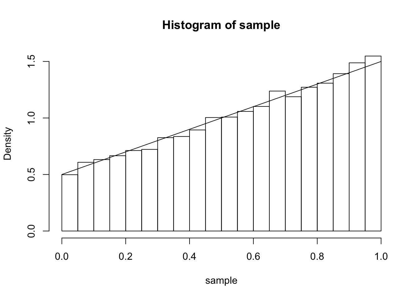
1. Using the inverse transform method, write an R function to generate a random variable with the distribution function \(F(x) = \frac{x^2+x}{2},0\le x\le 1\) Produce a histogram of samples drawn from this distribution and superimpose the density function.

I calculated that the inverse function is given by \(F^{-1}(x)=\frac{-1+\sqrt{1+8x}}{2},0\le x\le 1\)

I also calculated the density as \(x+\frac{1}{2}\)

DIST1 <- function(n) {
  u <- runif(n)
  X <- (-1+sqrt(1+8*u))/2
  return(X)
}

sample <- DIST1(10000)
hist(sample, probability = TRUE)
curve(x+1/2,add = TRUE)

Figure 1: Output of Question 1.

Q2

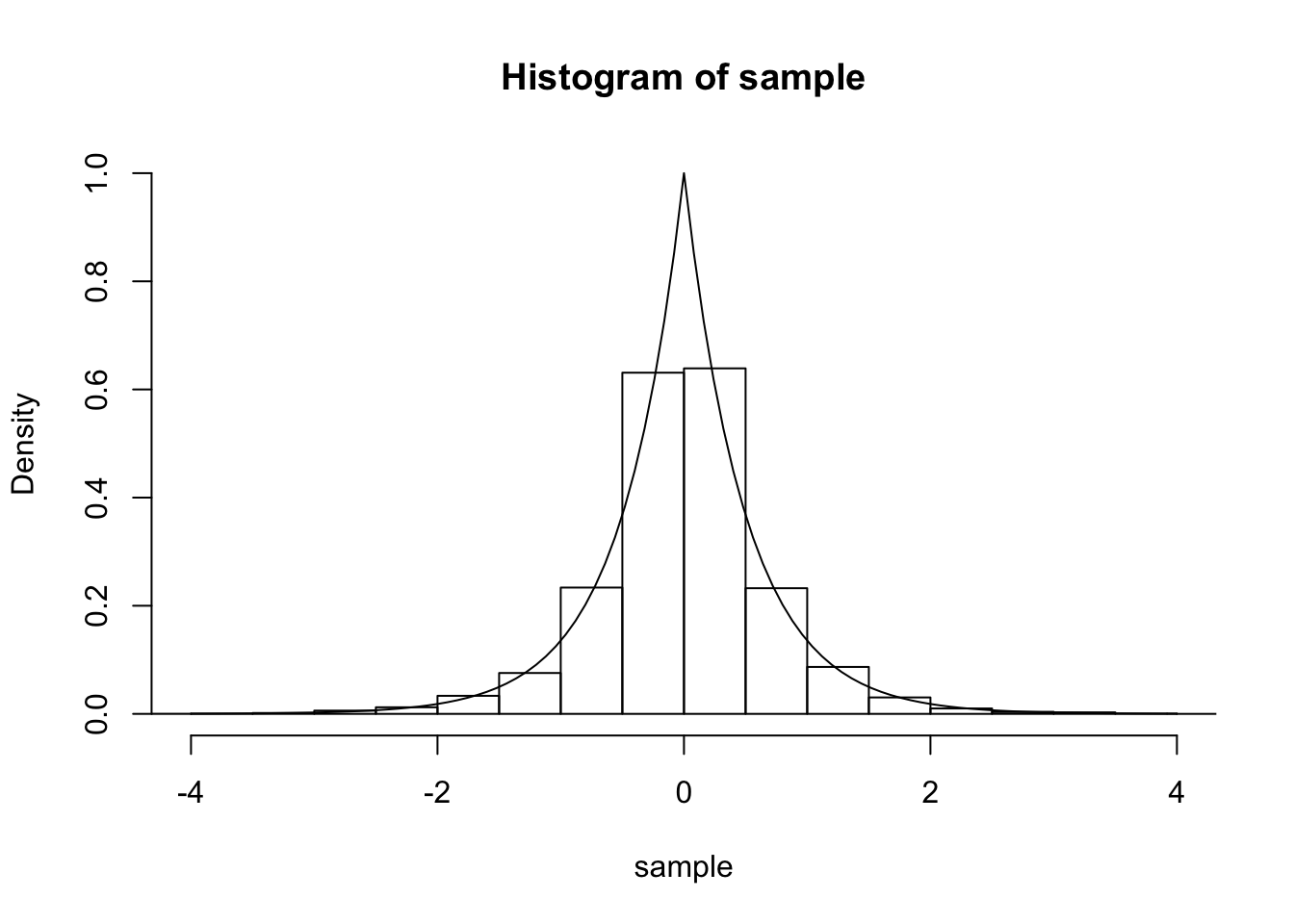
Using the inverse transform method, write an R function to generate a random variable with density function \(f(x) = \left\{ \begin{array}{ll} e^{2x} & \quad -\infty < x < 0 \\ e^{-2x} & \quad 0 \leq x < \infty \end{array} \right.\)

Produce a histogram of samples drawn from this distribution and superimpose the density function.

inverse2scalar <- function(x) {
  if (x < 1/2) {
    return(log(2*x)/2)
  }
  else {
    return(-1/2 *log(2-2*x))
  }
}
inverse2 <- Vectorize(inverse2scalar)

density2scalar <- function(x) {
  if (x < 0) {
    return(exp(2*x))
  }
  else {
    return(exp(-2*x))
  }
}
density2 <- Vectorize(density2scalar)

DIST2 <- function(n) {
  u <- runif(n)
  X <- inverse2(u)
  return(X)
}

sample <- DIST2(10000)
hist(sample, probability = TRUE, ylim=c(0,1), xlim=c(-4,4))
curve(density2(x), add = TRUE)

Figure 2: Output of Question 2.

Q3

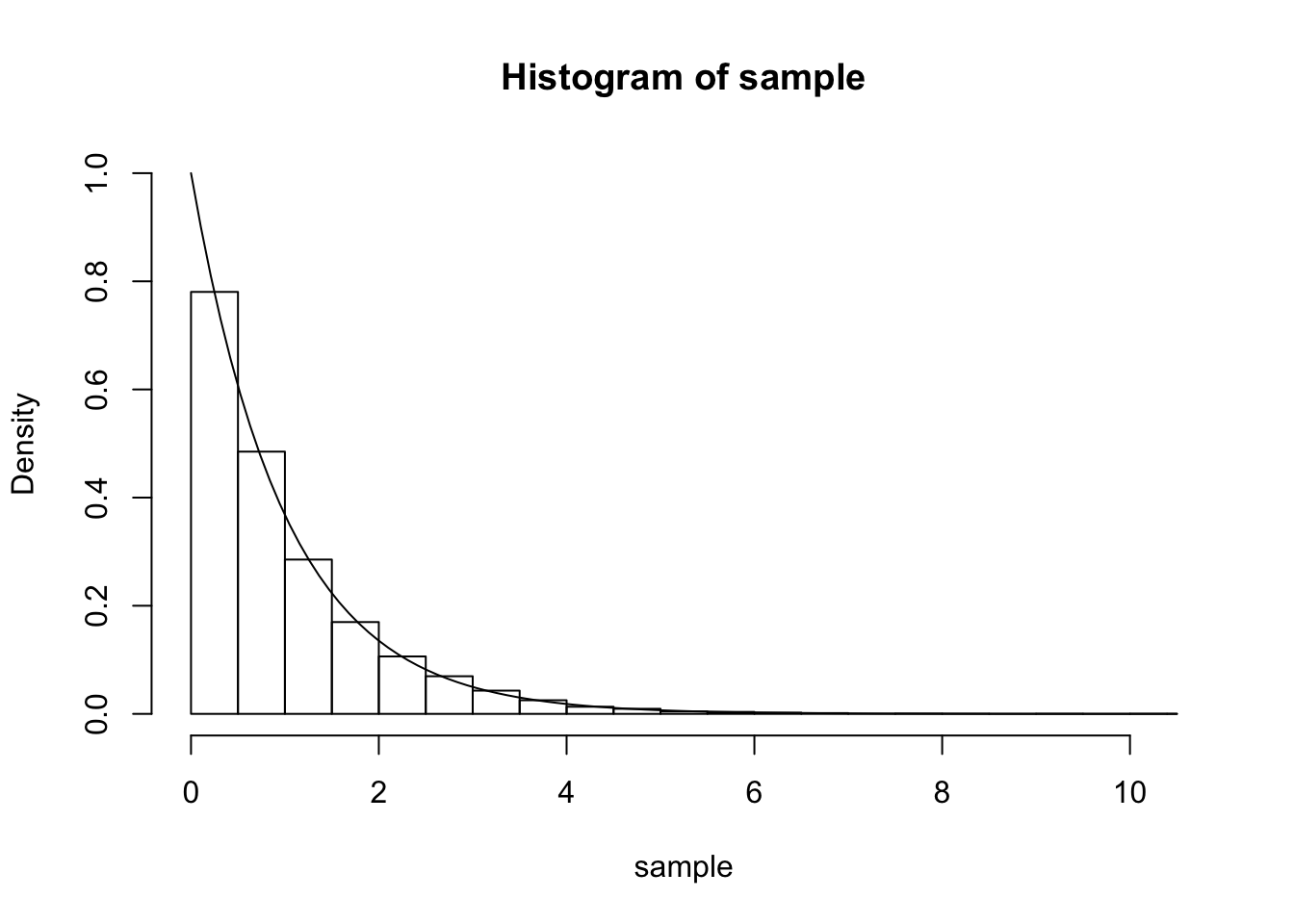
Using the probability integral transform method, write an R function to generate n ran- dom samples from an Exponential distribution \(x=e^{\lambda}\) Produce a histogram of samples drawn from this distribution and superimpose the density function. How large should you choose \(n\) for the approximation to be reasonable?

inverse3scalar <- function(x,lambda) {
  return(-1/lambda * log(1-x))
}
inverse3 <- Vectorize(inverse3scalar)

density3scalar <- function(x, lambda) {
  return(lambda*exp(-lambda*x))
}
density3 <- Vectorize(density3scalar)

DIST3 <- function(n, lambda) {
  u <- runif(n)
  X <- inverse3(u, lambda)
  return(X)
}

LAMBDA <- 1
N <- 10000
sample <- DIST3(N, LAMBDA)
hist(sample, probability = TRUE, ylim=c(0,LAMBDA))
curve(density3(x, LAMBDA), add = TRUE)

Figure 3: Output of Question 3.